Going between DLT <-> intrinsic/extrinsic: experimental data

Here we’ll go through using experimentally derived DLT coefficients. The DLT coefficients were derived using the easyWand tool. Three TeAx ThermalCapture thermal cameras were placed in a cave to record bat activity. Here, we’ll be tracking a falling object and checking to see if our measured gravitational accelaration matches the expected 9.8 \(m/s^{2}\).

References

• DLT to/from intrinsic+extrinsic https://biomech.web.unc.edu/dlt-to-from-intrinsic-extrinsic/ acc 2022-03-08

• http://www.kwon3d.com/theory/dlt/dlt.html#3d

Author: Thejasvi Beleyur, March 2022

import glob
import cv2
import matplotlib.pyplot as plt
from mpl_toolkits.mplot3d import Axes3D
import pandas as pd
import numpy as np
from track2trajectory.camera import Camera
from dlt_reconstruction_easyWand import dlt_reconstruct
from track2trajectory.synthetic_data import make_rotation_mat_fromworld, get_cam_centre_from_projectionmat
from track2trajectory.dlt_to_world import transformation_matrix_from_dlt, cam_centre_from_dlt
import mat73
from scipy.spatial import distance
from gravity_alignment import smooth_and_acc, row_calc_norm
# sphinx_gallery_thumbnail_path = '_static//threed_coordinates.png'
concat = np.concatenate

def point2point_matrix(xyz):
    distmat = np.zeros((xyz.shape[0],xyz.shape[0]))
    for i in range(distmat.shape[0]):
        for j in range(distmat.shape[1]):
            distmat[i,j] = distance.euclidean(xyz[i,:], xyz[j,:])
    return distmat

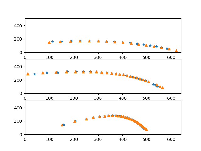
Undistorting pixel coordinates

Most, if not all, cameras have some form of distortion. Once we know the distortion coefficients, it is easy to ‘undistort’ an image or an object’s pixel coordinates, and thus generate corrected object coordinates.

# load the raw 2D tracking data
multicam_xy = pd.read_csv('DLTdv7_data_gravityxypts.csv')
colnames = multicam_xy.columns
cam1_2d, cam2_2d, cam3_2d = [multicam_xy.loc[:,colnames[each]].to_numpy(dtype='float32') for each in [[0,1], [2,3], [4,5]]]

# the pixel data was digitised using DLTdv (https://biomech.web.unc.edu/dltdv/)
# The image origin in DLTdv is set to the lower left. DO NOT shift them - or the DLT
# coefficients won't make sense anymore!!!!

cam1_2d[:,1] = cam1_2d[:,1] # edited legacy code. Previously this hadd 511 - cam1_2d[:,1]
cam2_2d[:,1] = cam2_2d[:,1]
cam3_2d[:,1] = cam3_2d[:,1]

know the intrinsic matrix (common to all cameras)

# camera image is 640 x 512
px,py = 320, 256
fx, fy = 526, 526 # in pixels

Kteax = np.array([[fx, 0, px],
                  [0, fy, py],
                  [0, 0,  1]])

same undistortion to all of them.

p1, p2 = np.float32([0,0]) # tangential distortion
k1, k2, k3 = np.float32([-0.3069, 0.1134, 0]) # radial distortion
dist_coefs = np.array([k1, k2, p1, p2, k3]) #in the opencv format

# apply undistortion now
cam1_undist = cv2.undistortPoints(cam1_2d, Kteax, dist_coefs, P=Kteax)
cam2_undist = cv2.undistortPoints(cam2_2d, Kteax, dist_coefs, P=Kteax)
cam3_undist = cv2.undistortPoints(cam3_2d, Kteax, dist_coefs, P=Kteax)

plt.figure()
plt.subplot(311)
plt.plot(cam1_2d[:,0], cam1_2d[:,1],'*')
plt.plot(cam1_undist[:,:,0], cam1_undist[:,:,1],'^')
plt.ylim(0,512)
plt.xlim(0,640)

plt.subplot(312)
plt.plot(cam2_2d[:,0], cam2_2d[:,1],'*')
plt.plot(cam2_undist[:,:,0], cam2_undist[:,:,1],'^')
plt.ylim(0,512)
plt.xlim(0,640)

plt.subplot(313)
plt.plot(cam3_2d[:,0], cam3_2d[:,1],'*')
plt.plot(cam3_undist[:,:,0], cam3_undist[:,:,1],'^')
plt.ylim(0,512)
plt.xlim(0,640)

plt.savefig('../docs/source/_static/undistorted_cameracoods.png')

DLT reconstruction using 11 parameter DLT from easyWand

fname = '2018-08-17_wand_dvProject.mat'

data_dict = mat73.loadmat(fname)
dltcoefs = data_dict['udExport']['data']['dltcoef']

c1_dlt, c2_dlt, c3_dlt = [dltcoefs[:,col] for col in [0,1,2]]


coefficents = np.column_stack((c1_dlt, c2_dlt))
xyz_easywand = []
for c1_pt, c2_pt in zip(cam1_undist[11:24], cam2_undist[11:24]):
    points = np.append(np.float32(c1_pt), np.float32(c2_pt)).reshape(1,-1)
    xyz_easywanddlt = dlt_reconstruct(coefficents, points)
    xyz_easywand.append(xyz_easywanddlt[0])
xyz_dlt_easywand = np.array(xyz_easywand).reshape(-1,3)

DLT -> Transformation-> Projection matrix

First we get the transformation matrix from the DLT coefficients and then following the Ty Hedrick and Taila Weiss write-ups here we’ll get the final projection matrix \(P\).

Handedness is important

It is important to know that different packages may have different handed coordinate systems - especially in the rotation matrices. In our case, the output from transfromation_matrix_from_dlt (a Python port of DLTcameraPosition) gives a rotation matrix with a right-handed system. We need ‘flip’ the rotation matrix to get sensible xyz coordinates.

shifter_mat = np.row_stack(([1,0,0,0],
                            [0,1,0,0],
                            [0,0,-1,0],
                            [0,0,0,1]))

T1, _, ypr1 = transformation_matrix_from_dlt(dltcoefs[:,0])
T2, _, ypr2 = transformation_matrix_from_dlt(dltcoefs[:,1])
T3, _, ypr3 = transformation_matrix_from_dlt(dltcoefs[:,2])

# shift the whole transformation matrix  and then
# extract the 3x3 rotation matrix out
shifted_rotmat1 = np.matmul(T1, shifter_mat)[:3,:3]
shifted_rotmat2 = np.matmul(T2, shifter_mat)[:3,:3]
shifted_rotmat3 = np.matmul(T3, shifter_mat)[:3,:3]

# Use world camera centre and camera rotation matrix
# to make world->camera transformation matrix
T1cam = make_rotation_mat_fromworld(shifted_rotmat1, T1[-1,:3])
T2cam = make_rotation_mat_fromworld(shifted_rotmat2, T2[-1,:3])
T3cam = make_rotation_mat_fromworld(shifted_rotmat3, T3[-1,:3])

m = np.column_stack((np.eye(3), np.zeros(3))) # the 3x4 matrix to 'grease the wheels'

P11kmt = np.matmul(Kteax, np.matmul(m,T1cam))
P22kmt = np.matmul(Kteax, np.matmul(m,T2cam))
P33kmt = np.matmul(Kteax, np.matmul(m,T3cam))

cam1 = Camera(1, [0,0,0], fx, px, py, fx, fy, Kteax, [0,0,0],
              np.eye(3), np.zeros(5), [0,0,0], P11kmt)
cam2 = Camera(2, [0,0,0], fx, px, py, fx, fy, Kteax, [0,0,0],
              np.eye(3), np.zeros(5), [0,0,0], P22kmt)
cam3 = Camera(2, [0,0,0], fx, px, py, fx, fy, Kteax, [0,0,0],
              np.eye(3), np.zeros(5), [0,0,0], P33kmt)

xyz_Tmat_based = []
for c1_pt, c2_pt in zip(cam1_undist[11:24], cam2_undist[11:24]):
    position_homog = cv2.triangulatePoints(P11kmt, P22kmt,
                                           c1_pt.flatten(), c2_pt.flatten())
    xyz_Tmat_based.append(cv2.convertPointsFromHomogeneous(position_homog.T))

xyz_Tmat_based = np.array(xyz_Tmat_based).reshape(-1,3)

Generate projection matrix from DLT coefficients

This is based on my attempts at trying to recreate the projection matrix \(P\) directly from the DLT coefficients (again inspired by the Hedrick lab link)

def extract_P_from_dlt_v2(dltcoefs):
    '''No normalisation
    '''
    dltcoefs = np.append(dltcoefs, 1)
    dltcoefs = dltcoefs

    P = dltcoefs.reshape(3,4)
    return P

# generate projection matrix
Pcam1 = extract_P_from_dlt_v2(c1_dlt)
Pcam2 = extract_P_from_dlt_v2(c2_dlt)

# Now get 3D positions using cv2.triangulatePositions
xyz_P_based = []
for pt1, pt2 in zip(cam1_undist[11:24,:], cam2_undist[11:24,:]):
    pt1_homog, pt2_homog = (X.reshape(1,1,2) for X in [pt1, pt2])
    position = cv2.triangulatePoints(Pcam1, Pcam2, pt1_homog, pt2_homog)
    final_xyz = cv2.convertPointsFromHomogeneous(position.T).flatten()
    xyz_P_based.append(final_xyz)

xyz_P_based = np.array(xyz_P_based).reshape(-1,3)

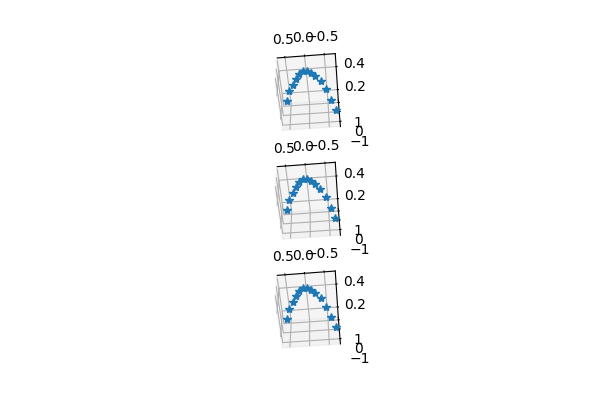
Visualise all of these points - we see the parabolic path of an object that’s been thrown and is falling as it flies through the air.

plt.figure(figsize=(6,4))
ax = plt.subplot(311, projection='3d')
ax.view_init(azim=95, elev=-54)
ax.plot(xyz_dlt_easywand[:,0],
        xyz_dlt_easywand[:,2],
        xyz_dlt_easywand[:,1], '*')
ax2 = plt.subplot(312, projection='3d')
ax2.view_init(azim=95, elev=-54)
ax2.plot(xyz_Tmat_based[:,0], xyz_Tmat_based[:,2], xyz_Tmat_based[:,1], '*')
ax3 = plt.subplot(313, projection='3d')
ax3.view_init(azim=95, elev=-54)
ax3.plot(xyz_P_based[:,0], xyz_P_based[:,2], xyz_P_based[:,1], '*')

plt.savefig('../docs/source/_static/threed_coordinates.png')

How similar or dissilimar are the points. They may have different origins and axis orientations - but the euclidean distances between points should remain the same

indices = np.arange(13)
pbased_distmat = point2point_matrix(xyz_P_based[indices,:])
tbased_distmat = point2point_matrix(xyz_Tmat_based[indices,:])
easywand_distmat = point2point_matrix(xyz_dlt_easywand[indices,:])

Camera centres across the different methods DLT based method (code from Ty Hedrick)

Ccam1_dltmethod = cam_centre_from_dlt(dltcoefs[:,0])
Ccam2_dltmethod = cam_centre_from_dlt(dltcoefs[:,1])
intercam_dist_dlt = distance.euclidean(Ccam1_dltmethod, Ccam2_dltmethod)

Ccam1_Pmethod = get_cam_centre_from_projectionmat(Pcam1)
Ccam2_Pmethod = get_cam_centre_from_projectionmat(Pcam2)
intercam_dist_P = distance.euclidean(Ccam1_Pmethod, Ccam2_Pmethod)

print(f'Inter-camera centre distance: \n Projection mat: {intercam_dist_P}\n DLT method: {intercam_dist_dlt}')

Get the overall accelaration. This is a falling object, and so the only accelaration should be the gravitational accelaration ~9.8 \(m/s^{2}\)

acc_dlt = smooth_and_acc(xyz_dlt_easywand,fps=25)
acc_P = smooth_and_acc(xyz_P_based, fps=25)
acc_tmat = smooth_and_acc(xyz_Tmat_based,fps=25)

here (%age of g)

relative_mean_acc = np.array([np.mean(each)/9.81 for each in [row_calc_norm(acc_dlt), row_calc_norm(acc_P), row_calc_norm(acc_tmat)]])

print(f'g has been estimated to within {relative_mean_acc*100} \
      of its true value with the 3 methods')

using the three methods.

plt.figure()
plt.plot(row_calc_norm(acc_dlt),'-.' ,label='dlt reconstruction')
plt.plot(row_calc_norm(acc_P), '^', label='Projection matrix based')
plt.plot(row_calc_norm(acc_tmat), label='projection from T matrix')
plt.hlines(9.8, 0,10,'k', label='g=9.81 $m/s^{2}$')
plt.legend();plt.ylim(8,10.5)

plt.savefig('../docs/source/_static/g_acc.png')

get_range = lambda X: np.max(X) - np.min(X)

def get_stack_absdiff(XXX):
    return np.apply_along_axis(get_range, 2, XXX)

rows, cols = pbased_distmat.shape
all_distmats = np.zeros((rows, cols, 3))
all_distmats[:,:,0] = pbased_distmat
all_distmats[:,:,1] = tbased_distmat
all_distmats[:,:,2] = easywand_distmat

distmat_range = get_stack_absdiff(all_distmats)

print(f'Max range in distance matrices across \
      3 methods: {np.max(distmat_range)}')